scope basics III : Plotting an array

this tutorial demonstrates how to plot an array with a horizontal axis linked to the array index (through triggering) using the plot command and the scope tool. It also shows how to use run-time YOS scripting for manipulating array variables and their content.

info

• Let's presume that a successful comlink with the device was already established (the device is connected, connection options were set, the driver was installed, etc.)
• Let's presume that you are familiar with the YOS scripting.

tip

• For more information, check the scope manual page.

• A good practice is to start the scope tool first (before setting up the on-board sampling service). That way, the scope will adjust itself according to the captured plot setup, (legend, scale, units, descriptions ...). The plot setup is streamed out from the device only when you are assigning a new variable to sample through plot.

Using the term

First, open the term and log in. We will walk through a few code snippets below. You can copy-paste them into the terminal window to try.

Making the arrays

There are not many array variables commonly present in the device. So, let's make some in the run-time. We will start with creating two arrays as dynamic varaibles, each composed of 100 floating point numbers:

var array1.100 array2.100 float

We may already plot those. Nevertheless, YOS variables are auto-initialized to zero upon creation. Let's fill them up with some more interesting content first. How about a single period of sine and cosine wave :

var i
var amplitude frequency t float
set amplitude 1
set frequency 6.283185 # 2*PI
set t i 0
{
 set array1.$i amplitude*sin(t)
 set array2.$i amplitude*cos(t)

 set t t+(frequency:100)
 set i i+1

 if i<100 branch s
}

Let's print our arrays out at this point, to see what we got :

vr array1 array2

Plotting the arrays

The first array starts with zero and goes up, whereas the second array starts with one and goes down then. This suggests we have evaluated a sine and cosine wave. Let's now start the scope tool (if you haven't already, to start capturing the data). Then, plot these as an array using the command:

plot -a array1 array2

Bring the scope window to the top. Make sure that the scroll flag is not checked, as now we want Left-to-right sample ordering and press enter to auto-adjust the scales. You may zoom in to see the data. The array data should look like this:

tip

By default, the plot will keep updating the graph. If you want to have a single-shot depiction, add -o option.

info

If we treat the depicted array as an external sample buffer and implement a triggerable sampling process within the device, the sampling rate limit is no longer coupled to the throughput of the chosen communications interface (as in the case of the periodic sampling). In this way, high sampling frequencies are possible. Such an approach is used for exp for the identrun process. Please contact siliXcon if you are interested in monitoring some onboard processes with higher sampling rates.

Continuous update

The array graphs are now continuously updated. Hence, if the array content in the device changes, the graph also changes. Let's use that feature and modify our code to change the content continuously. The code below is an amalgamation of the snippets from above. The loop has been modified to be infinite and to constantly evaluate the sin and cos functions into the arrays:

# make and plot our arrays
var array1.100 array2.100 float
plot -c -a array1 array2 # the -c flag clears the plot (if a sampling is already assigned)

# make some more variables needed for the generation
var i
var amplitude frequency t float
set t i 0


# initialize values of the sine wave parameters
set amplitude 1
set frequency 6.283185 # 2*PI

# begin the loop
{
 set array1.$i amplitude*sin(t)
 set array2.$i amplitude*cos(t)

 set t t+(frequency:100)
 set i i+1

 if i<100 branch s

 ########
 # The following two lines were added to start over (when arrays are full) and make the loop infinite

 set t i 0
 branch s
}

At this moment, both waveforms are constantly being regenerated inside the device. The term will not respond to the enter since YOS/Shell is executing the infinite loop (until you terminate it with ctrl+C). However, you may still use emGUI or_yosctl_ to control the device.

tip

If you want to continue using the shell (e.g. to set amplitude and frequency), even when a script is running, make it detached by adding & after the latest code block character (see YOS manual).

To play with the sine wave graph, let's run emGUI now (either with ctrl+g or from LaunchPad and initiate Search). Navigate to /vars directory and you will see the variables we just created. Double-click on frequency and amplitude to bring up their dialogs.

info

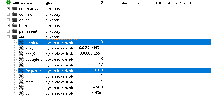
If you already have the emGUI running, you need to fetch the tree again (in the /vars folder) to see the newly created variables.

Now, you can play with the frequency and amplitude values and watch the sine-wave being updated in run-time. We essentially created a simple, parametric sine-wave generator.

tip

• Note that all the computation is happening onboard the device; therefore, it is easy to integrate real measurements as well as connect your calculations to the real device output.
• You may also use yosctl to manipulate all the variables programmatically.