scope
is a Matlab-inspired simple tool for real-time data graphing.
Multiple instances of the scope can run. There are up to 4 plots inside a scope. Each plot can hold up to 8 trends.
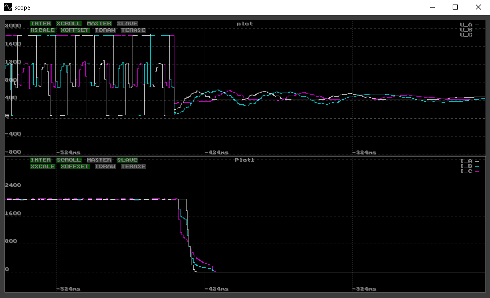 A close-up view of block commutation, showing voltages and currents in a BLDC motor.
Functional description
To maximize real-time performance, scope was designed as a passive tool. Therefore, it doesn't control sampling itself nor the time-base of the process. The scope captures and displays incoming samples from a comlink.
I want to set up my sampling!
To control the sampling service, use dedicated YOS commands. These can be invoked via term (or emGUI, SXapi, yosctl ...) :
plot- rich command for setting up the sample base, timing and parameters.period- an alias for sampling period adjustment.legend- additional visual-style scope control (axis description, legend, trend colors, name of the figure ...).
If one of the plots in the scope is closed and the sampling service still runs on the device, the plot is re-opened automatically. To close it permanently, the sampling service has to be stopped in the device first.
Scope saves its actual setting. When the scope is run again, it is opened with the latest settings.
Capture trigger
Normally, an incoming sample triggers the capture immediately. If one of the plot frames has the SLAVE flag set, the incoming sample is not written to the corresponding buffer immediately. Instead, it is written only when a sample from a plot with MASTER arrives. In this way, un-even sampling can be synchronized according to one, common capture trigger.
The user can pause the global capture with space on the keyboard.
Capture ordering
scope is built around a sample buffer. Similarly to a digital oscilloscope, it displays the content of the sample buffer as a graph.
Depending on the scrolling flag, the incoming samples may be stored in the buffer in two manners:
-
Left-to-right. Each new sample increments the index. When the end of the buffer is reached, or when a trigger signal arrives, the index is reset to zero and new samples are written from the beginning again. If the
TERASEflag is set, the buffer is cleared at this moment. If theTDRAWflag is set, the graph is drawn only at this moment. This mode is usually preferred when monitoring an indirect, triggerable process or an external sample array. -
Scrolling. Each new sample is pushed at the end of the buffer and the remaining samples are shifted by one position to the left. This mode is usually preferred when monitoring a continuous, time-dependent process with periodic sampling.
There may be up to 8 values inside the incoming sample. These values are further regarded as different trends. The underlying transfer protocol automatically determines the data type (int8, int16, float, ...).
Horizontal axis notion
as mentioned earlier, the horizontal axis does not strictly denote time, contrary to common assumptions. Instead of adding time stamps to incoming samples, scope avoids this due to potential distortions caused by communication jitter.
The axis actually only represents the index of the sample buffer. The precise time base is determined by the sampling service within the device, and users can adjust the sampling frequency, for example, using the period command.
In the Left-to-Right mode, the horizontal axis might correspond to the index of an externally maintained sample buffer. This approach is typically useful in scenarios where the sampling frequency exceeds the data transmission capacity of the communication link.
Data navigation
Scope purposefully doesn't attempt to interpolate the data in between samples. The zero-order-hold depiction is used to avoid confusion around measurand behavior in between the samples.
Vertical line link connection between samples can be toggled on and off with the INTER flag. A missing sample, stored as a floating-point NaN, is not displayed.
A keyboard and mouse can be used to crawl through the trends (adjust scales and offsets). The auto-set function will attempt to auto-adjust the scales and offsets of a single plot according to the data.
Setting XSCALE and XOFFSET within multiple plot frames will glue their X-axis scale and offset together.
Saving and loading the buffer
The user can save/load the sample buffer data to/from a .csv file upon request. Remarks:
- Each column corresponds to the trend's scalar sample value.
- Each row (line) corresponds to a single sample and each newline increments the pointer in the sample buffer. If no value is provided for a trend, a missing value is put onto its buffer.
- If a value starts with
#, it's string is not parsed out as a numeric value but interpreted as name of the trend.
The example of the content of a saved .csv file:
#temp;#2;#3;#4;#5;#6;#7;#8;
36.035072;;;;;;;;
36.038349;;;;;;;;
36.055431;;;;;;;;
36.024368;;;;;;;;
36.050514;;;;;;;;
36.062389;;;;;;;;
36.091965;;;;;;;;
36.073593;;;;;;;;
36.075691;;;;;;;;
Recording and playback of the samples
The user can initiate recording/playback of the samples. On the contrary to the saving/loading functionality, recording/playback is a continuous process and must be also terminated by the user on-demand. Remarks:
- The
.csvfile format is the same as described above, within the Saving and loading the data section. - In Recording mode, each captured sample is appended to a new line in the
.csvfile. - In Playback mode, the file is periodically checked for changes. If the file's modification time changes, the file is reloaded. All the samples are processed as if they would come from the device.
Offline mode
Scope can be started without being attached to the comlink with a device. In such mode, it can be used for exp. to explore previously recorded / saved data, or simply as a stand-alone .csv file data viewer.
Keyboard control
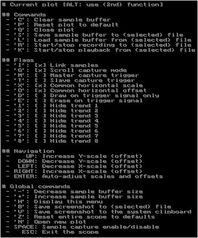
global
-- (minus) decrease sample memory size.+- (plus) increase sample memory size.h- display menu with available functions.b- save the current figure screenshot to a file. Combining withCtrlopens up a dialog to choose the file. Otherwise, a default filename will be used, or the last file will be overwritten.v- save the current figure screenshot to the system clipboard.z- reset the entire scope to defaults.n- open a new plot in the current scope window.Space- global data sampling enable/disable (pauses and runs the data capture).Esc- exit the scope.Tab- switche between the plots in the current scope window.F1toF4- select the plot 1 to 4.
per Plot frame
c- clear current plot data.p- reset the current plot to default settings.q- close the current plot.s- save current plot data to a file - save actual sample buffer the.csvfile. Combining withCtrlopens up a dialog to choose the file. Otherwise, a default filename will be used, or the last file will be overwritten.l- load data from a file to the current plot - load data from a.csvfile to the sample buffer. Combining withCtrlopens up a dialog to choose the file. Otherwise, a default filename will be used, or the last file will be overwritten.r- start/stop real-time recording to a file - record/stop captured samples to the.csvfile. Combining withCtrlopens up a dialog to choose the file. Otherwise, a default filename will be used, or the last file will be overwritten.k- start/stop real-time playback from a file - play/stop captured samples from the.csvfile. Combining withCtrlopens up a dialog to choose the file. Otherwise, a default filename will be used, or the last file will be overwritten.
data navigation
Up/Downarrows,mouse scroll up/down- scale Y-scale.Left/Rightarrows,mouse scroll left/right,Ctrl + mouse scroll up/down- scale X-scale.Ctrl + Up/Downarrows,mouse clickand drag - offset Y-offset.Ctrl + Left/Rightarrows,mouse clickand drag - offset X-offset.Enter- auto-adjust scales and offsets according to current sample data.
The following flags can be toggled on and off by pressing the corresponding key or by clicking buttons in the upper left corner of each plot frame:
e- toggle the 'erase plot on trigger signal'.d- toggle the 'redraw plot on trigger signal only'.o- toggle the 'common X-axis offset' - plot frames with this function toggled on will have the same offset of the X-axis.x- toggle the 'common X-axis scale' - plot frames with this function toggled on will have the same scale on the X-axis.t- toggle the 'slave capture' - capture trigger of this plot is synchronized with the master plot (described below).m- toggle the 'master capture' - capture trigger of this plot is taken as reference for all plot frames with the slave flag toggled on.g- toggle the 'scrolling plot' - when toggled off, the plot is drawn from the left to the right. The oldest data in the memory are rewritten by the newest ones. When toggled on, the plot is running from right to left. With each sample, data are shifted by one position.i- toggle the 'link samples' - when toggled on, measured points are connected with a vertical line, depicting the Zero-order-hold representation, when toggled off, only sample points without lines are displayed.- Numbers
1to8- toggle trends 1 to 8.
Mouse control
By clicking inside an allocated plot, it gains focus. The plot-specific keyboard shortcuts are directed to the focused plot.
Data navigation
Drag and drop will adjust the offsets. The user can also toggle the flags in the left-top corner (described above). Mouse wheel and Ctrl + mouse wheel will control the horizontal and vertical zoom. Modern touchpads should control zoom through multi-finger scrolling in both directions.
Cursor
By left-clicking anywhere inside in an allocated plot, a cursor appears to assist with data read-out (only when the drag and drop did not occur). The cursor is anchored to a particular value and sample position in the sample buffer. Upon clicking again to the same place, cursor will disappear.

Menu
A simple, markdown-styled menu can be opened by right-clicking anywhere inside the scope window. The menu offers the same functions as the above-mentioned keyboard shortcuts.
Automated control
The legend YOS command may be used for controlling the scope tool from inside the device, e.g. using scripting. Apart from all the controls hereby specified, legend can also enrich the graph visualization with:
- specifying units of the axes,
- setting scale factor of the axes,
- setting trend line color and line style,
- describing the individual trends,
- labeling the plot,
- labeling the entire window.